The basic equation of antigravity

Dmitry Ponomarev V.

Saint-Petersburg, Russia

20.01.2025

The main characteristic of the gravitational field of a material body is its gravitational potential. Moreover, the value of the gravitational potential of the field at a specific point in space does not give an idea of the direction of the gravitational force, it is necessary to determine the potential difference of the gravitational field ∆φ in order to unambiguously indicate the direction of the gravitational force. It is known that the force of gravitational interaction is directed towards decreasing the gravitational potential of the field and perpendicular to the tangent to the equipotential surface of the gravitational field of a material body, i.e. ∆φ positive:

Equation (1)

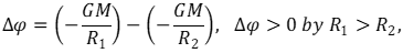
where: ∆φ – is the potential difference of the gravitational field of a body with a rest mass M; R1 and R2 – are the distance from a material body with a rest mass M; G – is the gravitational constant.

Equation (1) describes the direction of the gravitational force vector of the gravitational field. This force is commonly referred to as the force of gravitational interaction. Therefore, it is logical to state that the force of the antigravity interaction should be described by the following equation (i.e. ∆φ is negative):

Equation (1)

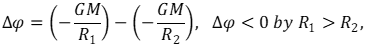
Thus, we can say that an equation of the form (2) is the basic equation of antigravity, since it describes the direction of the vector of gravitational force in the direction away from the material body forming the gravitational field.

Now let’s consider the mechanism for obtaining the antigravity interaction of bodies and write down the basic equation of antigravity in more detail in accordance with the parameters of this interaction. It should be noted that further in the work a rotating reference frame with a constant angular velocity of rotation w will be considered and only gravitational forces are subject to consideration. All other forces (fictitious forces [1]) arising in a rotating frame of reference (centrifugal force, Coriolis force and Euler force) are not considered in this work.

Figure 1 shows a material body with a rest mass M with two equipotential surfaces 1 and 2, as well as a disk rotating with a constant angular velocity ω (blue line). The distance from the center of the point mass M to the disk along the axis of rotation of the disk is H, the radius of the disk is r. On the disk, we select for consideration one of the points m (particle m) at a distance r from the axis of rotation.

In this paper, the rotating disk is considered as an antigravity wing (AGW), the definition of which can be found in [2].

An accelerated moving particle does not have an inertial frame of reference (a rotating frame of reference is not inertial), in which it is always at rest. However, it is always possible to find an inertial reference frame that is currently moving with the particle. This system is called the “momentarily comoving reference frame” (MCRF) and allows the application of special relativity theory to analyze motion ([3], [4]). It is with this particle m (the point m on the disk) that we associate the reference frame S, which is indicated in Figure 1 by the red dotted lines of the x and y coordinate axes. From this frame of reference, we will observe physical processes. Since point m is an integral and integral part of the entire disk, and it is stationary with respect to every other point on the disk, including the center of the disk, the reference frame S is connected to the reference frame of the disk S’ (for example, with the triangle Mom with the coordinate axes x and y’ in Figure 1), and more precisely, they have the same angular velocity of rotation ω relative to a body with a rest mass M.

Figure 1 – The mechanism of obtaining antigravity interaction of bodies

Two articles of the relativistic model of antigravity interaction of bodies are devoted to a more detailed consideration of various reference systems and the possibility of applying relativistic transformations in them: “Reference systems for antigravity interaction of bodies” [5] and “Manifestation of gravitational and antigravity fields depending on the reference system” [6].

The relativistic gravitational potential of a body M at point m (along the equipotential surface 1) will be equal to:

Equation (3)

where: c – is the speed of light in a vacuum.

The cosine of the angle α between r and R is:

Equation (4)

In order to determine the potential difference ∆φ of the gravitational field of a body M, it is necessary to determine the second equipotential surface with which the gravitational potential at point m will be compared. Let’s choose the equipotential surface furthest from the point m, which is in contact with the disk – this is the equipotential surface 2. The choice of this second equipotential surface for analysis is justified by the fact that if an antigravity interaction is recorded in the space between these two equipotential surfaces, then, consequently, antigravity will be observed between all other points along the radius of the disk and point m relative to the observation from point m.

Then the distance between the two equipotential surfaces will be equal to dR. Since the triangle Mom rotates with an angular velocity ω, the triangle uem also rotates with an angular velocity ω, and therefore the angular velocity at point u is equal to the angular velocity at point e.

Therefore, the relativistic gravitational potential of the body M at point u (along the equipotential surface 2 at a distance H from the body M) will be equal to:

Equation (5)

Since dr is equal to:

Equation (6)

Then equation (5) is written as:

Equation (7)

Since ∆φ = φ1 – φ2, then:

Equation (8)

Equation (8) could be called the basic equation of antigravity, but so far there is still a lack of definition at which values of angular velocity ω the condition ∆φ<0 will be fulfilled. Next, we will determine these values of ω, but first we will illustrate equation (8) on a graph based on terrestrial conditions (the Earth is represented with a spherically symmetric mass distribution).

For calculations, we take the following values: c = 3∙108 m/s, G = 6,67∙10-11 N∙m2/kg2, M = 6∙1024 kg (Earth’s mass), H = 6,37∙106 m (Earth’s radius), i.e. the disk will rotate near the Earth’s surface.

Next, the angular velocity ω will be expressed as follows:

Equation (9)

where: n – is the number of revolutions per second.

To illustrate the calculations, we take n = 38000 revolutions per second and consider all points (particles) of the rotating disk (including point m) along the radius of the disk r (r is conventionally taken equal to 1000 m), i.e. we get a graph of the function ∆φ(r), which is shown in Figure 2.

Figure 2 – Graph of the function of the difference in gravitational field potentials

Figure 3 – Zones of gravitational and antigravity interaction

In Figure 2, one can observe not only the gravitational and antigravity interaction of point m (particle m) with a material body M, but also all other points (particles) of a rotating disk along the radius of disk r with this body M, i.e. passing through all equipotential surfaces from the axis of rotation of the disk to point m. For a visual interpretation of the resulting graph of the function ∆φ(r), we introduce symbols and zones, which are shown in Figure 3.

Let’s analyze the calculated data, but once again recall that the graph of the function ∆φ(r) in Figure 3 shows the difference in gravitational potentials between a point on the disk at a distance of r and a point located towards the center of the body M on the equipotential surface 2 (for example, for point m, this is pointing u in Figure 1):

1. For radius r = 0 (point a) ∆φ=0. This result is understandable, since in the absence of the radius r, the disk itself is missing (there is nothing to consider);
2. Along the segment ac, there is a positive difference in gravitational potentials (∆φ>0) – this corresponds exactly to equation (1), i.e. there is a gravitational interaction (even on the segment bc);
3. At point c, the gravitational potential difference ∆φ=0, which means that weightlessness is observed at point c. This point itself is conventionally called the zero-gravity point (rn);
4. There is already a negative difference in gravitational potentials in the cd segment (∆φ<0), and it is this part of the disk that will provide the overall resultant force, which will first partially compensate for the gravitational force, and then repel the disk from the material body M. This part of the disk is the so-called useful area of the antigravity wing, which works to repel material bodies from each other. It is worth noting that the initial point m (Figure 1) is located at point d (Figure 3). The very point c+dr, where dr→0, is conventionally called the antigravity point (ra), i.e. This is the point at which, with a further increase in the distance r from which or an increase in the angular velocity ω, the antigravity interaction begins to be observed (∆φ<0).

Now let us determine at which values of the angular velocity ω the condition 0>∆φ will be fulfilled (i.e. ∆φ is negative) in equation (8), i.e.:

Equation (10)

Converting equation (10) taking into account equation (9), we obtain the angular velocity ω and then the rotational frequency n, at which the point m will repel from the material body M:

Equation (11)

Equation (12)

As a result, from equations (8) and (11) we write:

Equation (13)

Since H – is the distance from the center of the point mass M to the disk along the axis of rotation of the disk, and it is also the distance to the equipotential surface 2, and taking into account the legend R through R1 and H through R2, we write down the basic equation of antigravity in general form, which can be used to analyze the difference in gravitational potentials between any two equipotential surfaces.

The basic equation of antigravity:

Equation (14)

The angular velocity ω can be used to express the linear velocity υ, which will be at a distance r from the axis of rotation (υ is equal to the product of r by ω):

Equation (15)

The ratio of the indicated velocity υ to the speed of light c will be equal to:

Equation (16)

Using the basic antigravity equation (14), it is possible to determine the required rotation frequency of the disk (antigravity wing) for its complete location in the antigravity field relative to the observation point m (i.e., observing from a distance r from the axis of rotation). Here are a number of calculated examples based on real data, which are presented in Table 1.

Table 1 - The required rotation frequency of the antigravity wing for its complete location in the Earth’s antigravity field relative to the observation point at a distance r from the axis of rotation

As can be seen from Table 1, a relatively small increase in the radius of the disk (antigravity wing) leads to a significant reduction in the required rotation frequency. However, in any case, the instantaneous linear velocity at the edge of the antigravity wing (at point m) should be about 70.7% of the speed of light. This value gives an idea of the level of speeds that must be dealt with in order to possibly achieve antigravity.

An increase in the ratio of linear velocity to the speed of light is also visible with an increase in the radius of the antigravity wing (in table 1, this is noted at the 5-7 decimal places). What this means and why it happens is additionally described in the work “The Point of antigravity” [7] of the relativistic model of antigravity interaction of bodies.

In conclusion, it should be noted that this work is a development of the relativistic model of antigravity interaction of bodies [8] and has not only theoretical but also practical significance, since the results of the work make it possible to determine the necessary rotation frequency of the antigravity wing to overcome the gravitational force of the Earth. We make an important point that an antigravity wing in practical implementation does not necessarily have to and will not be represented as a classical metal (or other material) disk, as we present it above in the drawings describing the antigravity interaction of bodies, although it is convenient for a theoretical description of the principle of antigravity implementation, since it reflects a classical rotating frame of reference.

References:

1. Rotating reference frame. – URL: https://en.wikipedia.org/wiki/Rotating_reference_frame (date of request: 14.07.2025).
2. Ponomarev D. The main theses and definitions of the relativistic model of antigravity interaction of bodies. – URL: https://antigravity-theory.ru/antigravity-theses (date of request: 14.07.2025).
3. Relativistic Doppler effect. – URL: https://en.wikipedia.org/wiki/Relativistic_Doppler_effect (date of request: 14.07.2025).
4. Proper reference frame (flat spacetime). – URL: https://en.wikipedia.org/wiki/Proper_reference_frame_(flat_spacetime) (date of request: 14.07.2025).
5. Ponomarev D. Reference frames for antigravity interaction of bodies. – URL: https://antigravity-theory.ru/antigravity-reference-frames-2 (date of request: 14.07.2025).
6. Ponomarev D., Shibeko R. The manifestation of gravitational and antigravity fields depending on the frame of reference. – URL: https://antigravity-theory.ru/antigravity-reference-frames (date of request: 14.07.2025).
7. Ponomarev D. The antigravity point. – URL: https://antigravity-theory.ru/antigravity-point (date of request: 14.07.2025).
8. Antigravity. Relativistic model of antigravity interaction of bodies. – URL: https://antigravity-theory.ru (date of request: 14.07.2025).

© Ponomarev D., 2025

antigravity-theory@yandex.ru