Obesity is a multifactorial condition with genetic, environmental, and behavioral causes. In this community, obesity prevalence is significantly higher in specific ZIP codes, indicating a possible health disparity (ie, preventable health differences associated with social, environmental, or economic disadvantage).
Obesity-related health disparities represent a major public health concern with increased prevalence, severity, and complications affecting vulnerable communities. Such disparities involve factors relating to health care (eg, provider screening and treatment, access to care), patients (eg, diet and activity, health knowledge), and neighborhood (eg, density of
grocery stores, which influences dietary patterns; crime rate, which influences physical activity).
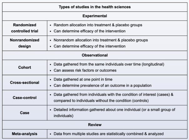
Given the multifactorial nature of obesity and related disparities, the first step in researching this community's trend is to generate hypotheses. This is best achieved through cross- sectional analysis of demographic and behavioral data, which is relatively easy to perform and can depict multiple risk factors at one point in time (a "snapshot") to:
- reveal differences in distribution (prevalence) of demographic factors (eg, poverty, ethnicity, insurance status) across ZIP codes.
- identify variables correlated (associated) with obesity risk (eg, poverty is more prevalent in high-obesity ZIP codes).
- generate hypotheses (eg, poverty increases obesity risk by decreasing ability to consume foods promoting optimal weight).
Other study designs are more appropriate for testing or refining hypotheses following broader cross-sectional analysis.
(Choices B and D) Like cross-sectional analysis, cohort studies and qualitative surveys offer observational data for generating hypotheses. However, each of these approaches focuses on a single, patient-related hypothesis (eg, leptin, patient knowledge and attitudes) for obesity differences. Cross-sectional analysis involving this community's demographic factors is a better first step, as it can analyze multiple potential influences and tailor hypotheses to this setting.
(Choice C) Quality improvement studies analyze and test clinical processes (eg, providing obesity screening) affecting health care quality. They are less useful for generating broad hypotheses for community epidemiological patterns (eg, obesity trends).
(Choice E) Randomized controlled trials are more appropriate for testing (rather than generating) hypotheses; such trials would be premature at this stage. Moreover, this approach tests only health care factors whereas cross-sectional analysis can assess how other risk factors correlate to obesity risk in this community.
Important parameters of diagnostic tests include the following:
- True positives (TP) represent diseased individuals with positive test results.
- True negatives (TN) represent healthy individuals with negative test results.
- False positives (FP) represent healthy individuals with positive test results.
- False negatives (FN) represent diseased individuals with negative test results.
- Sensitivity (TP/ [TP + FN]) represents a test's ability to correctly identify diseased individuals from among all individuals. A test with high sensitivity has a low FN rate (important for screening purposes). With a highly sensitive test, most diseased patients will have a positive test result (and a negative test result would help rule out the disease [SnNOut]).
- Specificity (TN/ [TN + FP]) represents the ability of a test to exclude those without the disease. A very specific test has a low FP rate (important for confirmatory tests). With a highly specific test, most healthy patients will have a negative test result (and a positive test result would help rule in the disease [SpPIn]).
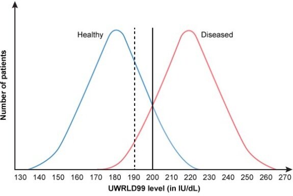
The cutoff value of a quantitative diagnostic test determines whether a given result is interpreted as positive or negative. Depending on the disease or condition being tested for, sensitivity or specificity may be preferred and the cutoff value adjusted accordingly. A cutoff value just outside the overlapping region of the curves can maximize the sensitivity or specificity at 100% by correctly classifying all diseased or healthy individuals, respectively.
In the above example, changing the cutoff point to a lower value (shift to the left) would cause
more patients with the disease to test positive (↑TP, ↓FN), increasing the sensitivity of the
test. However, as a consequence, more patients without the disease would also test positive
(↓TN, ↑FP), resulting in decreased specificity.
(Choices A, D, and E) Raising the cutoff value (shift to the right) would cause fewer individuals with the disease to have a positive test result (↓TP, ↑FN), so sensitivity would decrease. Fewer individuals without the disease would also test positive (↑TN, ↓FP), so specificity would increase.
(Choice B) Positive predictive value (PPV = TP / [TP + FP]) represents the probability that a patient with a positive test result actually has the disease. In this case, the lower cutoff value would increase both TP and FP; how this affects the PPV depends on disease prevalence, which is not provided. In a population with very low disease prevalence, the number of FP would be expected to increase proportionately more than the number of TP, which would lower the PPV.
Case control study
A case-control study is the most appropriate study design for evaluating the public health officials' claim. This is because the disease (acute myelogenous leukemia [AML]) is a rare condition occurring at a higher rate in this population, and a retrospective exposure (chemical waste exposure) needs to be evaluated. In case-control studies, 2 groups of subjects are created: cases (subjects with the disease of interest) and controls (subjects without the disease of interest). After the case and control groups are selected, exposure frequency to a specific variable (eg, chemical waste) within both groups is ascertained. If there is a statistically significant difference in exposure frequency between the 2 groups, it is likely that the variable in question is associated with disease development.
In this example, AML is the disease of interest; therefore, children with AML should be used as cases and children without AML should be used as controls. Cases and controls should be selected regardless of exposure status to the chemical waste (Choices A and B). Selecting
subjects based on exposure status is inappropriate because comparing the frequency of exposure between the case and control groups is what determines whether the exposure is more prevalent among cases as compared to controls.
Ideally, exposure frequency among controls should be representative of that among the population of individuals "at risk" of becoming cases. In other words, for a given case-control study, controls are nondiseased individuals who could be considered cases if they had the disease. Often, controls and cases are matched based on independent variables (eg, age, sex) to decrease the effects of confounding.
(Choices D, E, and F) AML is the outcome of interest; therefore, children who have AML can be used only to form the cases group and cannot be used as controls. Cases should also be selected regardless of exposure status.
Confounding occurs when the exposure-disease relationship is muddled by the effect of a confounding variable, an extraneous factor associated with both exposure and disease. An example is shown in the exhibit. In a primary school, it may appear on crude analysis that students with bigger shoe sizes have a higher level of intelligence. However, this association is actually a result of age, not shoe size: Older students tend to have bigger shoe sizes and also to be more intelligent. Age is a confounder because it is associated with both shoe size and intelligence and muddles the association between them. When study subjects are grouped by age (stratification), the association between shoe size and intelligence is no longer significant.
Similarly, initial crude analysis suggested that alcohol use was associated with bladder carcinoma (similar to shoe size being associated with intelligence), with a relative risk (RR) of
1.81 and a p-value <0.05. However, smoking is associated with both bladder carcinoma and alcohol use. Therefore, smoking is a potential confounder that may explain the association observed between alcohol use and bladder cancer (similar to age in the school
example). Stratified analysis by smoking status shows that both smokers and non-smokers have an RR ~1 with large p-values (>0.05). The RR of 1.81 found on crude analysis disappears
and there is no true association between alcohol consumption and bladder cancer.
(Choice B) Effect modification results when an external variable positively or negatively impacts the observed effect of a risk factor on disease status. When analysis is performed
based on stratification by this external variable, there will be a significant difference in risk between the stratified groups. For instance, aspirin use is associated with Reye syndrome in children but not adults; therefore, age modifies the effect of aspirin on Reye syndrome development. Effect modification can easily be confused with confounding; but stratified analysis can help distinguish between them. With confounding, there is usually no significant difference between the strata (as in this case with the smoker and non-smoker strata).
(Choices C and E) Measurement bias and observer bias distort the strength of association by misclassifying exposed/unexposed and/or diseased/nondiseased subjects. The scenario does not describe any issues that could affect the classification process.
(Choice D) Meta-analysis refers to compiling results from several studies to increase analysis power.
(Choice F) Recall bias results from inaccurate recall of past exposure by people in the study and applies mostly to retrospective (eg, case-control) studies.
Researchers develop a new test to detect the presence of a recently identified biomarker for hepatocellular carcinoma (HCC). The initial evaluation of the test shows the following:
Which of the following is the likelihood that a patient with a negative test does not have HCC? Ans)
The negative predictive value (NPV) of a diagnostic test is the probability (ie, likelihood) that an individual truly does not have the disease given a negative test. It is equal to the number of individuals who do not have the disease and who have a negative test result (ie, true negatives [TN]) divided by the total number of individuals with a negative test result (TN + false negatives [FN]). Therefore, NPV is calculated as:
NPV = TN / (TN + FN)
In this example, 120 individuals are TN and 5 individuals are FN; therefore, the total number of individuals with a negative test result (TN + FN) is 125 (ie, 120 + 5), and the test's NPV is calculated as follows:
NPV = TN / (TN + FN) = 120 / (120 + 5) = 120 / 125 = 0.96
Positive and negative predictive values depend on the prevalence of the disease in the study population. For example, it is more likely that individuals who test positive truly have the disease and less likely that individuals who test negative do not have the disease in a high- prevalence population compared to a low-prevalence population.
(Choice A) 0.10 is the false negative rate (FNR). FNR is equal to FN / (FN + TP) and describes the proportion of the individuals who really have the disease for which the test result is negative. It is also known as the miss rate.
(Choice B) 0.20 is the false positive rate (FPR). FPR is equal to FP / (FP + TN) and describes the proportion of the individuals who really do not have the disease for which the test result is positive. It is also known as the fall-out rate.
(Choice C) 0.60 is the overall proportion of TN in the entire study: TN / (TP + TN + FP + FN).
(Choice D) 0.80 is the test's specificity. Specificity is equal to TN / (TN + FP) and describes the proportion of individuals who do not have the disease for which the test result is negative. It is an intrinsic measure of the test's ability to correctly identify individuals without the disease, but by itself, it does not provide enough information to interpret a negative test result in a particular individual.
The cutoff value of a quantitative diagnostic test determines whether a given result is interpreted as positive or negative. When there is overlap between the serum values of the healthy and diseased populations, a cutoff value that correctly categorizes all individuals in both populations cannot be chosen. This limits the sensitivity and specificity of the test due to the presence of false positive (FP) and/or false negative (FN) individuals.
Sensitivity represents the ability of a test to correctly identify those with a given disease. It is calculated as the number of patients correctly testing positive (TP) divided by the total number
of patients with the disease (TP / [TP + FN]). Specificity represents the ability of a test to correctly identify those without a given disease. It is calculated as the number of patients correctly testing negative (TN) divided by the total number of patients without the disease (TN / [TN + FP]).